Solving the derivative for dummies: definition, how to find, examples of solutions. Derivatives of basic elementary functions Derivatives of elementary functions of the proof

Here is a summary table for convenience and clarity when studying the topic.

Let us analyze how the formulas of the indicated table were obtained, or, in other words, we will prove the derivation of formulas for derivatives for each type of function.

Derivative of a constant

In order to derive this formula, we take as a basis the definition of the derivative of a function at a point. We use x 0 = x, where x takes on the value of any real number, or, in other words, x is any number from the domain of the function f (x) = C . Let's write the limit of the ratio of the increment of the function to the increment of the argument as ∆ x → 0:

lim ∆ x → 0 ∆ f (x) ∆ x = lim ∆ x → 0 C - C ∆ x = lim ∆ x → 0 0 ∆ x = 0

Please note that the expression 0 ∆ x falls under the limit sign. It is not the uncertainty of “zero divided by zero”, since the numerator contains not an infinitesimal value, but zero. In other words, the increment of a constant function is always zero.

So, the derivative of the constant function f (x) = C is equal to zero over the entire domain of definition.

Example 1

Given constant functions:

f 1 (x) = 3 , f 2 (x) = a , a ∈ R , f 3 (x) = 4 . 13 7 22 , f 4 (x) = 0 , f 5 (x) = - 8 7

Decision

Let us describe the given conditions. In the first function we see the derivative of the natural number 3 . In the following example, you need to take the derivative of a, where a- any real number. The third example gives us the derivative of the irrational number 4 . 13 7 22 , the fourth - the derivative of zero (zero is an integer). Finally, in the fifth case, we have the derivative of the rational fraction - 8 7 .

Answer: the derivatives of the given functions are zero for any real x(over the entire domain of definition)

f 1 " (x) = (3) " = 0 , f 2 " (x) = (a) " = 0 , a ∈ R , f 3 " (x) = 4 . 13 7 22 " = 0 , f 4 " (x) = 0 " = 0 , f 5 " (x) = - 8 7 " = 0

Power function derivative

We turn to the power function and the formula for its derivative, which has the form: (x p) " = p x p - 1, where the exponent p is any real number.

Proof 2

Here is the proof of the formula when the exponent is a natural number: p = 1 , 2 , 3 , …

Again, we rely on the definition of a derivative. Let's write the limit of the ratio of the increment of the power function to the increment of the argument:

(x p) " = lim ∆ x → 0 = ∆ (x p) ∆ x = lim ∆ x → 0 (x + ∆ x) p - x p ∆ x

To simplify the expression in the numerator, we use Newton's binomial formula:

(x + ∆ x) p - x p = C p 0 + x p + C p 1 x p - 1 ∆ x + C p 2 x p - 2 (∆ x) 2 + . . . + + C p p - 1 x (∆ x) p - 1 + C p p (∆ x) p - x p = = C p 1 x p - 1 ∆ x + C p 2 x p - 2 (∆ x) 2 + . . . + C p p - 1 x (∆ x) p - 1 + C p p (∆ x) p

Thus:

(x p) " = lim ∆ x → 0 ∆ (x p) ∆ x = lim ∆ x → 0 (x + ∆ x) p - x p ∆ x = = lim ∆ x → 0 (C p 1 x p - 1 ∆ x + C p 2 x p - 2 (∆ x) 2 + . . . + C p p - 1 x (∆ x) p - 1 + C p p (∆ x) p) ∆ x = = lim ∆ x → 0 (C p 1 x p - 1 + C p 2 x p - 2 ∆ x + . . . + C p p - 1 x (∆ x) p - 2 + C p p (∆ x) p - 1) = = C p 1 x p - 1 + 0 + 0 + . . . + 0 = p! 1! (p - 1)! x p - 1 = p x p - 1

So, we proved the formula for the derivative of a power function when the exponent is a natural number.

Proof 3

To give proof for the case when p- any real number other than zero, we use the logarithmic derivative (here we should understand the difference from the derivative of the logarithmic function). To have a more complete understanding, it is desirable to study the derivative of the logarithmic function and additionally deal with the derivative of an implicitly given function and the derivative of a complex function.

Consider two cases: when x positive and when x are negative.

So x > 0 . Then: x p > 0 . We take the logarithm of the equality y \u003d x p to the base e and apply the property of the logarithm:

y = x p ln y = ln x p ln y = p ln x

At this stage, an implicitly defined function has been obtained. Let's define its derivative:

(ln y) " = (p ln x) 1 y y " = p 1 x ⇒ y " = p y x = p x p x = p x p - 1

Now we consider the case when x- a negative number.

If the indicator p is an even number, then the power function is also defined for x< 0 , причем является четной: y (x) = - y ((- x) p) " = - p · (- x) p - 1 · (- x) " = = p · (- x) p - 1 = p · x p - 1

Then xp< 0 и возможно составить доказательство, используя логарифмическую производную.

If a p is an odd number, then the power function is defined for x< 0 , причем является нечетной: y (x) = - y (- x) = - (- x) p . Тогда x p < 0 , а значит логарифмическую производную задействовать нельзя. В такой ситуации возможно взять за основу доказательства правила дифференцирования и правило нахождения производной сложной функции:

y "(x) \u003d (- (- x) p) " \u003d - ((- x) p) " \u003d - p (- x) p - 1 (- x) " = \u003d p (- x) p - 1 = p x p - 1

The last transition is possible because if p is an odd number, then p - 1 either an even number or zero (for p = 1), therefore, for negative x the equality (- x) p - 1 = x p - 1 is true.

So, we have proved the formula for the derivative of a power function for any real p.

Example 2

Given functions:

f 1 (x) = 1 x 2 3 , f 2 (x) = x 2 - 1 4 , f 3 (x) = 1 x log 7 12

Determine their derivatives.

Decision

We transform part of the given functions into a tabular form y = x p , based on the properties of the degree, and then use the formula:

f 1 (x) \u003d 1 x 2 3 \u003d x - 2 3 ⇒ f 1 "(x) \u003d - 2 3 x - 2 3 - 1 \u003d - 2 3 x - 5 3 f 2 "(x) \u003d x 2 - 1 4 = 2 - 1 4 x 2 - 1 4 - 1 = 2 - 1 4 x 2 - 5 4 f 3 (x) = 1 x log 7 12 = x - log 7 12 ⇒ f 3 "( x) = - log 7 12 x - log 7 12 - 1 = - log 7 12 x - log 7 12 - log 7 7 = - log 7 12 x - log 7 84

Derivative of exponential function

We derive the formula for the derivative, based on the definition:

(a x) " = lim ∆ x → 0 a x + ∆ x - a x ∆ x = lim ∆ x → 0 a x (a ∆ x - 1) ∆ x = a x lim ∆ x → 0 a ∆ x - 1 ∆ x = 0 0

We got uncertainty. To expand it, we write a new variable z = a ∆ x - 1 (z → 0 as ∆ x → 0). In this case a ∆ x = z + 1 ⇒ ∆ x = log a (z + 1) = ln (z + 1) ln a . For the last transition, the formula for the transition to a new base of the logarithm is used.

Let's perform a substitution in the original limit:

(a x) " = a x lim ∆ x → 0 a ∆ x - 1 ∆ x = a x ln a lim ∆ x → 0 1 1 z ln (z + 1) = = a x ln a lim ∆ x → 0 1 ln (z + 1) 1 z = a x ln a 1 ln lim ∆ x → 0 (z + 1) 1 z

Recall the second wonderful limit and then we get the formula for the derivative of the exponential function:

(a x) " = a x ln a 1 ln lim z → 0 (z + 1) 1 z = a x ln a 1 ln e = a x ln a

Example 3

The exponential functions are given:

f 1 (x) = 2 3 x , f 2 (x) = 5 3 x , f 3 (x) = 1 (e) x

We need to find their derivatives.

Decision

We use the formula for the derivative of the exponential function and the properties of the logarithm:

f 1 "(x) = 2 3 x" = 2 3 x ln 2 3 = 2 3 x (ln 2 - ln 3) f 2 "(x) = 5 3 x" = 5 3 x ln 5 1 3 = 1 3 5 3 x ln 5 f 3 "(x) = 1 (e) x" = 1 e x " = 1 e x ln 1 e = 1 e x ln e - 1 = - 1 e x

Derivative of a logarithmic function

We present the proof of the formula for the derivative of the logarithmic function for any x in the domain of definition and any valid values ​​of the base a of the logarithm. Based on the definition of the derivative, we get:

(log a x) " = lim ∆ x → 0 log a (x + ∆ x) - log a x ∆ x = lim ∆ x → 0 log a x + ∆ x x ∆ x = = lim ∆ x → 0 1 ∆ x log a 1 + ∆ x x = lim ∆ x → 0 log a 1 + ∆ x x 1 ∆ x = = lim ∆ x → 0 log a 1 + ∆ x x 1 ∆ x x x = lim ∆ x → 0 1 x log a 1 + ∆ x x x ∆ x = = 1 x log a lim ∆ x → 0 1 + ∆ x x x ∆ x = 1 x log a e = 1 x ln e ln a = 1 x ln a

It can be seen from the specified chain of equalities that the transformations were built on the basis of the logarithm property. The equality lim ∆ x → 0 1 + ∆ x x x ∆ x = e is true in accordance with the second remarkable limit.

Example 4

Logarithmic functions are given:

f 1 (x) = log log 3 x , f 2 (x) = log x

It is necessary to calculate their derivatives.

Decision

Let's apply the derived formula:

f 1 "(x) = (log ln 3 x)" = 1 x ln (ln 3) ; f 2 "(x) \u003d (ln x)" \u003d 1 x ln e \u003d 1 x

So the derivative of the natural logarithm is one divided by x.

Derivatives of trigonometric functions

We use some trigonometric formulas and the first wonderful limit to derive the formula for the derivative of a trigonometric function.

According to the definition of the derivative of the sine function, we get:

(sin x) " = lim ∆ x → 0 sin (x + ∆ x) - sin x ∆ x

The formula for the difference of sines will allow us to perform the following actions:

(sin x) " = lim ∆ x → 0 sin (x + ∆ x) - sin x ∆ x = = lim ∆ x → 0 2 sin x + ∆ x - x 2 cos x + ∆ x + x 2 ∆ x = = lim ∆ x → 0 sin ∆ x 2 cos x + ∆ x 2 ∆ x 2 = = cos x + 0 2 lim ∆ x → 0 sin ∆ x 2 ∆ x 2

Finally, we use the first wonderful limit:

sin "x = cos x + 0 2 lim ∆ x → 0 sin ∆ x 2 ∆ x 2 = cos x

So the derivative of the function sin x will cos x.

We will also prove the formula for the cosine derivative in the same way:

cos "x = lim ∆ x → 0 cos (x + ∆ x) - cos x ∆ x = = lim ∆ x → 0 - 2 sin x + ∆ x - x 2 sin x + ∆ x + x 2 ∆ x = = - lim ∆ x → 0 sin ∆ x 2 sin x + ∆ x 2 ∆ x 2 = = - sin x + 0 2 lim ∆ x → 0 sin ∆ x 2 ∆ x 2 = - sin x

Those. the derivative of the function cos x will be – sin x.

We derive the formulas for the derivatives of the tangent and cotangent based on the rules of differentiation:

t g "x = sin x cos x" = sin "x cos x - sin x cos "x cos 2 x = = cos x cos x - sin x (- sin x) cos 2 x = sin 2 x + cos 2 x cos 2 x = 1 cos 2 x c t g "x = cos x sin x" = cos "x sin x - cos x sin "x sin 2 x = = - sin x sin x - cos x cos x sin 2 x = - sin 2 x + cos 2 x sin 2 x = - 1 sin 2 x

Derivatives of inverse trigonometric functions

The section on the derivative of inverse functions gives comprehensive information on the proof of the formulas for the derivatives of the arcsine, arccosine, arctangent and arccotangent, so we will not duplicate the material here.

Derivatives of hyperbolic functions

We can derive formulas for the derivatives of the hyperbolic sine, cosine, tangent and cotangent using the differentiation rule and the formula for the derivative of the exponential function:

s h "x = e x - e - x 2" = 1 2 e x "- e - x" == 1 2 e x - - e - x = e x + e - x 2 = c h x c h "x = e x + e - x 2" = 1 2 e x "+ e - x" == 1 2 e x + - e - x = e x - e - x 2 = s h x t h "x = s h x c h x" = s h "x c h x - s h x c h "x c h 2 x = c h 2 x - s h 2 x c h 2 x = 1 c h 2 x c t h "x = c h x s h x" = c h "x s h x - c h x s h "x s h 2 x = s h 2 x - c h 2 x s h 2 x = - 1 s h 2 x

If you notice a mistake in the text, please highlight it and press Ctrl+Enter

Formulas 3 and 5 prove yourself.

BASIC RULES OF DIFFERENTIATION

Using the general method of finding the derivative using the limit, you can get the simplest differentiation formulas. Let be u=u(x),v=v(x) are two differentiable functions of a variable x.

Formulas 1 and 2 prove yourself.

Proof of Formula 3.

Let be y = u(x) + v(x). For argument value x+Δ x we have y(x+Δ x)=u(x+Δ x) + v(x+Δ x).

Δ y=y(x+Δ x) – y(x) = u(x+Δ x) + v(x+Δ x) – u(x) – v(x) = Δ u +Δ v.

Hence,

Proof of formula 4.

Let be y=u(x) v(x). Then y(x+Δ x)=u(x+Δ x)· v(x+Δ x), That's why

Δ y=u(x+Δ x)· v(x+Δ x) – u(x)· v(x).

Note that since each of the functions u and v differentiable at a point x, then they are continuous at this point, and hence u(x+Δ x)→u(x), v(x+Δ x)→v(x), for Δ x→0.

Therefore, we can write

Based on this property, one can obtain a rule for differentiating the product of any number of functions.

Let, for example, y=u v w. Then,

y " = u "·( v w) + u·( v w) "= u "· v w + u·( v" w + v w ") = u "· v w + u· v" w + u v w ".

Proof of Formula 5.

Let be . Then

In the proof, we used the fact that v(x+Δ x)→v(x) at Δ x→0.

Examples.

THEOREM ON THE DERIVATIVE OF A COMPLEX FUNCTION

Let be y = f(u), a u= u(x). We get a function y, depending on the argument x: y = f(u(x)). The last function is called a function of a function, or complex function.

Function scope y = f(u(x)) is either the entire scope of the function u=u(x) or that part of it in which the values ​​are determined u, not out of the scope of the function y= f(u).

The "function from function" operation can be performed not once, but any number of times.

Let us establish a rule for differentiating a complex function.

Theorem. If the function u= u(x) has at some point x0 derivative and takes the value at this point u 0 = u(x0), and the function y=f(u) has at the point u 0 derivative y"u= f "(u 0), then the complex function y = f(u(x)) at the specified point x0 also has a derivative, which is equal to y"x= f "(u 0)· u "(x0), where instead of u expression must be substituted u= u(x).

Thus, the derivative of a complex function is equal to the product of the derivative of this function with respect to the intermediate argument u to the derivative of the intermediate argument with respect to x.

Proof. For a fixed value X 0 we will have u 0 =u(x 0), at 0 =f(u 0 ). For new argument value x0+Δ x:

Δ u= u(x0 + Δ x) – u(x 0), Δ y=f(u 0+Δ u) – f(u 0).

Because u– differentiable at a point x0, then u is continuous at this point. Therefore, for Δ x→0 Δ u→0. Similarly, for Δ u→0 Δ y→0.

By condition . From this relation, using the definition of the limit, we obtain (for Δ u→0)

where α→0 at Δ u→0, and, consequently, for Δ x→0.

Let's rewrite this equation as:

Δ y=y"u ∆ u+α·Δ u.

The resulting equality is also valid for Δ u=0 for arbitrary α, since it turns into the identity 0=0. At Δ u=0 we will assume α=0. Divide all terms of the resulting equality by Δ x

.

By condition . Therefore, passing to the limit at Δ x→0, we get y"x= y" u u " x . The theorem has been proven.

So, to differentiate a complex function y = f(u(x)), you need to take the derivative of the "external" function f, treating its argument simply as a variable, and multiplying by the derivative of the "inner" function with respect to the independent variable.

If the function y=f(x) can be represented as y=f(u), u=u(v), v=v(x), then finding the derivative y " x is carried out by successive application of the previous theorem.

According to the proven rule, we have y"x= y"u · u" x . Applying the same theorem to u" x we ​​get , i.e.

y"x= y" x u"v · v"x= f"u( u)· u"v( v)· v"x( x).

Examples.

THE CONCEPT OF THE INVERSE FUNCTION

Let's start with an example. Consider the function y=x3. We will consider the equality y= x 3 as an equation for x. This is the equation for each value at defines a single value x: . Geometrically, this means that any line parallel to the axis Ox intersects the graph of the function y=x3 only at one point. Therefore we can consider x as a function of y. The function is called the inverse of the function y=x3.

Before passing to the general case, we introduce definitions.

Function y = f(x) called increasing on a certain interval, if the larger value of the argument x from this segment corresponds to a larger value of the function, i.e. if x 2 >x 1 , then f(x 2 ) > f(x 1 ).

Similarly, the function is called waning, if the smaller value of the argument corresponds to the larger value of the function, i.e. if X 2 < X 1 , then f(x 2 ) > f(x 1 ).

So, given an increasing or decreasing function y=f(x), defined on some interval [ a; b]. For definiteness, we will consider an increasing function (for a decreasing function, everything is similar).

Consider two different values X 1 and X 2. Let be y 1 =f(x 1 ), y 2 =f(x 2 ). It follows from the definition of an increasing function that if x 1 <x 2 , then at 1 <at 2. Therefore, two different values X 1 and X 2 correspond to two different function values at 1 and at 2. The opposite is also true, i.e. if at 1 <at 2 , then it follows from the definition of an increasing function that x 1 <x 2. Those. again to two different values at 1 and at 2 corresponds to two different values x 1 and x 2. Thus, between values x and their corresponding values y a one-to-one correspondence is established, i.e. the equation y=f(x) for everybody y(taken from the range of the function y=f(x)) defines a single value x, and we can say that x have some argument function y: x= g(y).

This function is called reverse for function y=f(x). Obviously, the function y=f(x) is the inverse of the function x=g(y).

Note that the inverse function x=g(y) is found by solving the equation y=f(x) relatively X.

Example. Let the function y= e x . This function increases at –∞< x <+∞. Она имеет обратную функцию x=ln y. Domain of the inverse function 0< y < + ∞.

Let's make some remarks.

Remark 1. If an increasing (or decreasing) function y=f(x) continuous on the segment [ a; b], and f(a)=c, f(b)=d, then the inverse function is defined and continuous on the segment [ c; d].

Remark 2. If the function y=f(x) is neither increasing nor decreasing on some interval, then it can have several inverse functions.

Example. Function y=x2 defined at –∞<x<+∞. Она не является ни возрастающей, ни убывающей и не имеет обратной функции. Однако, если мы рассмотриминтервал 0≤x<+∞, то здесь функция является возрастающей и обратной для нее будет . На интервале – ∞ <x≤ 0 the function is decreasing and its inverse .

Remark 3. If functions y=f(x) and x=g(y) are mutually inverse, then they express the same relationship between the variables x and y. Therefore, the graph is the same curve. But if we denote the argument of the inverse function again by x, and the function through y and build them in the same coordinate system, we get two different graphs. It is easy to see that the graphs will be symmetrical with respect to the bisector of the 1st coordinate angle.

THEOREM ON THE DERIVATIVE OF THE INVERSE FUNCTION

Let us prove a theorem that allows us to find the derivative of the function y=f(x) knowing the derivative of the inverse function.

Theorem. If for the function y=f(x) there is an inverse function x=g(y), which at some point at 0 has a derivative g "(v0) other than zero, then at the corresponding point x0=g(x0) function y=f(x) has a derivative f "(x0) equal to , i.e. correct formula.

Proof. Because x=g(y) differentiable at a point y 0, then x=g(y) is continuous at this point, so the function y=f(x) continuous at point x0=g(y 0). Therefore, for Δ x→0 Δ y→0.

Let us show that .

Let be . Then by the limit property . Let us pass in this equality to the limit at Δ y→0. Then Δ x→0 and α(Δx)→0, i.e. .

Hence,

,

Q.E.D.

This formula can be written as .

Let us consider the application of this theorem with examples.

We give without proof the formula for the derivatives of the basic elementary functions:

1. Power function: (x n)` =nx n -1 .

2. An exponential function: (a x)` = a x lna (in particular, (e x)` = e x).

3. Logarithmic function: (in particular, (lnx)` = 1/x).

4. Trigonometric functions:

(cosx)` = -sinx

(tgх)` = 1/cos 2 x

(ctgх)` = -1/sin 2 x

5. Inverse trigonometric functions:

It can be proved that in order to differentiate an exponential function, it is necessary to use the formula for the derivative of a complex function twice, namely, to differentiate it both as a complex exponential function and as a complex exponential function, and add the results: (f (x)  (x))` =(x)*f(x)  (x)-1 *f(x)` +f(x)  (x) *lnf(x)*(x)`.

Derivatives of higher orders

Since the derivative of a function is itself a function, it can also have a derivative. The concept of a derivative, which was discussed above, refers to a derivative of the first order.

derivativen-th order is called the derivative of the derivative of the (n-1)-th order. For example, f``(x) = (f`(x))` - second order derivative (or second derivative), f```(x) = (f``(x))` - third order derivative (or third derivative), etc. Sometimes Roman Arabic numerals in brackets are used to indicate higher derivatives, for example, f (5) (x) or f (V) (x) for a fifth-order derivative.

The physical meaning of derivatives of higher orders is defined in the same way as for the first derivative: each of them represents the rate of change of the derivative of the previous order. For example, the second derivative is the rate of change of the first, i.e. speed speed. For rectilinear motion, it means the acceleration of a point at a time.

Function elasticity

Function elasticity E x (y) is the limit of the ratio of the relative increment of the function y to the relative increment of the argument x with the latter tending to zero:
.

The elasticity of a function shows approximately how many percent the function y \u003d f (x) will change when the independent variable x changes by 1%.

In the economic sense, the difference between this indicator and the derivative is that the derivative has units of measurement, and therefore its value depends on the units in which the variables are measured. For example, if the dependence of the volume of production on time is expressed in tons and months, respectively, then the derivative will show the marginal increase in volume in tons per month; if, however, these indicators are measured, for example, in kilograms and days, then both the function itself and its derivative will be different. Elasticity is essentially a dimensionless value (measured in percentages or fractions) and therefore does not depend on the scale of indicators.

Basic theorems on differentiable functions and their applications

Fermat's theorem. If a function differentiable on an interval reaches its maximum or minimum value at an interior point of this interval, then the derivative of the function at this point is equal to zero.

Without proof.

The geometric meaning of Fermat's theorem is that at the point of the largest or smallest value achieved within the gap, the tangent to the graph of the function is parallel to the abscissa axis (Figure 3.3).

Rolle's theorem. Let the function y \u003d f (x) satisfy the following conditions:

2) differentiable on the interval (a, b);

3) takes equal values ​​at the ends of the segment, i.e. f(a)=f(b).

Then there is at least one point inside the segment where the derivative of the function is equal to zero.

Without proof.

The geometric meaning of Rolle's theorem is that there is at least one point at which the tangent to the graph of the function will be parallel to the x-axis (for example, there are two such points in Figure 3.4).

If f(a) =f(b) = 0, then Rolle's theorem can be formulated differently: between two successive zeros of a differentiable function there is at least one zero of the derivative.

Rolle's theorem is a special case of Lagrange's theorem.

Lagrange's theorem. Let the function y \u003d f (x) satisfy the following conditions:

1) is continuous on the segment [a, b];

2) is differentiable on the interval (a, b).

Then inside the segment there is at least one such point c at which the derivative is equal to the quotient of the increment of the functions divided by the increment of the argument on this segment:
.

Without proof.

To understand the physical meaning of Lagrange's theorem, we note that
is nothing else than the average rate of change of the function on the entire interval [a,b]. Thus, the theorem states that inside the segment there is at least one point at which the "instantaneous" rate of change of the function is equal to the average rate of its change over the entire segment.

The geometric meaning of Lagrange's theorem is illustrated in Figure 3.5. Note that the expression
is the slope of the line on which the chord AB lies. The theorem states that there is at least one point on the graph of a function at which the tangent to it will be parallel to this chord (i.e. the slope of the tangent - the derivative - will be the same).

Corollary: if the derivative of a function is equal to zero on some interval, then the function is identically constant on this interval.

In fact, let's take an interval on this interval. By Lagrange's theorem, there is a point c in this interval for which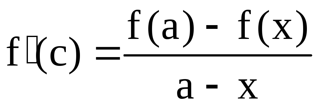
. Hence f(a) - f(x) = f`(с)(a - x) = 0; f(x) = f(a) = const.

L'Hopital's rule. The limit of the ratio of two infinitely small or infinitely large functions is equal to the limit of the ratio of their derivatives (finite or infinite), if the latter exists in the indicated sense.

In other words, if there is an uncertainty of the form
, then
.

Without proof.

The application of L'Hospital's rule to find limits will be covered in practical exercises.

A sufficient condition for the increase (decrease) of a function. If the derivative of a differentiable function is positive (negative) within some interval, then the function increases (decreases) on this interval.

Proof. Consider two values ​​x 1 and x 2 from the given interval (let x 2 > x 1). By Lagrand's theorem, on [x 1 , x 2 ] there is a point c at which
. Hence f (x 2) -f (x 1) \u003d f` (c) (x 2 -x 1). Then for f`(c) > 0, the left side of the inequality is positive, i.e. f(x 2) > f(x 1), and the function is increasing. At f`(s)< 0 левая часть неравенства отрицательна, т.е.f(х 2)

The theorem has been proven.

Geometric interpretation of the condition of monotonicity of the function: if the tangents to the curve in a certain interval are directed at acute angles to the abscissa axis, then the function increases, and if at obtuse angles, then it decreases (see Figure 3.6).

Remark: the necessary condition for monotonicity is weaker. If the function increases (decreases) on a certain interval, then the derivative is non-negative (non-positive) on this interval (i.e., at some points, the derivative of a monotone function can be equal to zero).

When deriving the very first formula of the table, we will proceed from the definition of the derivative of a function at a point. Let's take where x- any real number, that is, x– any number from the function definition area . Let us write the limit of the ratio of the function increment to the argument increment at :

It should be noted that under the sign of the limit, an expression is obtained, which is not the uncertainty of zero divided by zero, since the numerator contains not an infinitesimal value, but precisely zero. In other words, the increment of a constant function is always zero.

Thus, derivative of a constant functionis equal to zero on the entire domain of definition.

Derivative of a power function.

The formula for the derivative of a power function has the form , where the exponent p is any real number.

Let us first prove the formula for the natural exponent, that is, for p = 1, 2, 3, ...

We will use the definition of a derivative. Let us write the limit of the ratio of the increment of the power function to the increment of the argument:

To simplify the expression in the numerator, we turn to Newton's binomial formula:

Hence,

This proves the formula for the derivative of a power function for a natural exponent.

Derivative of exponential function.

We derive the derivative formula based on the definition:

Came to uncertainty. To expand it, we introduce a new variable , and for . Then . In the last transition, we used the formula for the transition to a new base of the logarithm.

Let's perform a substitution in the original limit:

If we recall the second remarkable limit, then we come to the formula for the derivative of the exponential function:

Derivative of a logarithmic function.

Let us prove the formula for the derivative of the logarithmic function for all x from the scope and all valid base values a logarithm. By definition of the derivative, we have:

As you noticed, in the proof, the transformations were carried out using the properties of the logarithm. Equality is valid due to the second remarkable limit.

Derivatives of trigonometric functions.

To derive formulas for derivatives of trigonometric functions, we will have to recall some trigonometry formulas, as well as the first remarkable limit.

By definition of the derivative for the sine function, we have .

We use the formula for the difference of sines:

It remains to turn to the first remarkable limit:

So the derivative of the function sin x there is cos x.

The formula for the cosine derivative is proved in exactly the same way.

Therefore, the derivative of the function cos x there is –sin x.

The derivation of formulas for the table of derivatives for the tangent and cotangent will be carried out using the proven rules of differentiation (derivative of a fraction).

Derivatives of hyperbolic functions.

The rules of differentiation and the formula for the derivative of the exponential function from the table of derivatives allow us to derive formulas for the derivatives of the hyperbolic sine, cosine, tangent and cotangent.

Derivative of the inverse function.

So that there is no confusion in the presentation, let's denote in the lower index the argument of the function by which differentiation is performed, that is, it is the derivative of the function f(x) on x.

Now we formulate rule for finding the derivative of the inverse function.

Let the functions y = f(x) and x = g(y) mutually inverse, defined on the intervals and respectively. If at a point there exists a finite non-zero derivative of the function f(x), then at the point there exists a finite derivative of the inverse function g(y), and . In another entry .

This rule can be reformulated for any x from the interval , then we get .

Let's check the validity of these formulas.

Let's find the inverse function for the natural logarithm (here y is a function, and x- argument). Solving this equation for x, we get (here x is a function, and y her argument). I.e, and mutually inverse functions.

From the table of derivatives, we see that and .

Let's make sure that the formulas for finding derivatives of the inverse function lead us to the same results:

As you can see, we got the same results as in the table of derivatives.

Now we have the knowledge to prove formulas for derivatives of inverse trigonometric functions.

Let's start with the derivative of the arcsine.

. Then, by the formula for the derivative of the inverse function, we obtain

It remains to carry out the transformation.

Since the range of the arcsine is the interval , then (see the section on basic elementary functions, their properties and graphs). Therefore, we do not consider.

Hence, . The domain of definition of the derivative of the arcsine is the interval (-1; 1) .

For the arccosine, everything is done in exactly the same way:

Find the derivative of the arc tangent.

For the inverse function is .

We express the arc tangent through the arc cosine to simplify the resulting expression.

Let be arctanx = z, then

Hence,

Similarly, the derivative of the inverse tangent is found:

The calculation of the derivative is often found in USE assignments. This page contains a list of formulas for finding derivatives.

Differentiation rules

1. (k⋅f(x))′=k⋅f′(x).
2. (f(x)+g(x))′=f′(x)+g′(x).
3. (f(x)⋅ g(x))′=f′(x)⋅ g(x)+f(x)⋅ g′(x).
4. Derivative of a complex function. If y=F(u) and u=u(x), then the function y=f(x)=F(u(x)) is called a complex function of x. Is equal to y′(x)=Fu′⋅ ux′.
5. Derivative of an implicit function. The function y=f(x) is called the implicit function given by the relation F(x,y)=0 if F(x,f(x))≡0.
6. Derivative of the inverse function. If g(f(x))=x, then the function g(x) is called the inverse function for the function y=f(x).
7. Derivative of a parametrically given function. Let x and y be given as functions of the variable t: x=x(t), y=y(t). It is said that y=y(x) is a parametrically defined function on the interval x∈ (a;b) if on this interval the equation x=x(t) can be expressed as t=t(x) and the function y=y( t(x))=y(x).
8. Derivative of exponential function. It is found by taking the logarithm to the base of the natural logarithm.