Find the empirical function according to the sample data. Empirical distribution function

Sample average.

Suppose that for the study of the general population with respect to the quantitative attribute X, a sample of volume n is extracted.

The sample mean is called the arithmetic mean of the attribute of the sample population.

Sample variance.

In order to observe the dispersion of the quantitative characteristic of the sample values ​​around its mean value, a summary characteristic is introduced - the sample variance.

Sample variance is the arithmetic mean of the squares of the deviation of the observed values ​​of the feature from their mean.

If all values ​​of the selection characteristic are different, then

Corrected variance.

Sample variance is a biased estimate of the general variance, i.e. the mathematical expectation of the sample variance is not equal to the estimated general variance, but is

To correct the sample variance, it is enough to multiply it by a fraction

Selective correlation coefficient is found by the formula

where are the sample standard deviations of the values ​​and.

The sample correlation coefficient shows the closeness of the linear relationship between and: the closer to one, the stronger the linear relationship between and.

23. A polygon of frequencies is a polyline whose segments connect points. To build a polygon of frequencies, the options are laid on the abscissa axis, and the frequencies corresponding to them on the ordinate axis, and the points are connected with straight line segments.

The polygon of relative frequencies is constructed in the same way, except that relative frequencies are plotted on the ordinate.

The frequency histogram is a stepped figure consisting of rectangles, the bases of which are partial intervals of length h, and the heights are equal to the ratio. To construct a histogram of frequencies on the abscissa axis, partial intervals are plotted, and above them, segments are drawn parallel to the abscissa axis at a distance (height). The area of ​​the i-th rectangle is equal to the sum of frequencies, the variant of the i-o interval, therefore the area of ​​the histogram of frequencies is equal to the sum of all frequencies, i.e. sample size.

Empirical distribution function

Where n x- the number of sampled values ​​less than x; n- sample size.

22 Let's define the basic concepts of mathematical statistics

.Basic concepts of mathematical statistics. General population and sample. Variational series, statistical series. Grouped sample. Grouped statistical series. Polygon of frequencies. Sampled distribution function and histogram.

General population- the whole set of available objects.

Sample- a set of objects randomly selected from the general population.

A sequence of variants, written in ascending order, is called variational next, and the list of options and their corresponding frequencies or relative frequencies - statistical series: tea selected from the general population.

Polygon frequencies are called a broken line, the segments of which connect the points.

Frequency histogram is called a stepped figure consisting of rectangles, the bases of which are partial intervals of length h, and the heights are equal to the ratio.

Sample (empirical) distribution function call the function F *(x), which determines for each value x relative frequency of the event X< x.

If some continuous feature is being investigated, then the variation series can consist of a very large number of numbers. In this case, it is more convenient to use pooled sample... To obtain it, the interval in which all the observed values ​​of the feature are enclosed is divided into several equal partial intervals of length h, and then find for each partial interval n i- the sum of the frequencies of the variant that fell into i th interval.

20. The law of large numbers should not be understood as any one general law associated with large numbers. The law of large numbers is a generalized name for several theorems, from which it follows that with an unlimited increase in the number of trials, the average values ​​tend to some constants.

These include the theorems of Chebyshev and Bernoulli. Chebyshev's theorem is the most general law of large numbers.

The proof of theorems, united by the term "law of large numbers", is based on Chebyshev's inequality, which establishes the probability of deviation from its mathematical expectation:

19 Pearson distribution (chi - square) - distribution of a random variable

where the random variables X 1, X 2, ..., X n independent and have the same distribution N(0.1). In this case, the number of terms, i.e. n is called the "number of degrees of freedom" of the chi-square distribution.

The chi-square distribution is used when estimating variance (using a confidence interval), when testing hypotheses of agreement, homogeneity, independence,

Distribution t Student's t is the distribution of a random variable

where the random variables U and X independent, U has a standard normal distribution N(0,1), and X- chi distribution - square with n degrees of freedom. Wherein n is called the "number of degrees of freedom" of the Student distribution.

It is used when evaluating the mathematical expectation, predicted value and other characteristics using confidence intervals, to test hypotheses about the values ​​of mathematical expectations, regression coefficients,

The Fisher distribution is the distribution of a random variable

The Fisher distribution is used to test hypotheses about the adequacy of the model in regression analysis, about the equality of variances, and in other problems of applied statistics.

18Linear regression is a statistical tool used to predict future prices based on past data and is commonly used to determine when prices are overheated. The least square method is used to plot the “best fit” straight line through a series of price points. The price points used as input can be any of the following values: open, close, high, low,

17. Two-dimensional random variable is an ordered set of two random variables or.

Example: Two dice are rolled. - the number of points dropped on the first and second dice, respectively

A universal way to define the law of distribution of a two-dimensional random variable is the distribution function.

15.m.o Discrete random variables

Properties:

1) M(C) = C, C- constant;

2) M(CX) = CM(X);

3) M(X 1 + X 2) = M(X 1) + M(X 2), where X 1, X 2- independent random variables;

4) M(X 1 X 2) = M(X 1)M(X 2).

The mathematical expectation of the sum of random variables is equal to the sum of their mathematical expectations, i.e.

The mathematical expectation of the difference of random variables is equal to the difference of their mathematical expectations, i.e.

The mathematical expectation of the product of random variables is equal to the product of their mathematical expectations, i.e.

If all values ​​of a random variable are increased (decreased) by the same number C, then its mathematical expectation will increase (decrease) by the same number

14. Exponential(exponential)distribution law X has an exponential (exponential) distribution law with parameter λ> 0, if its probability density has the form:

Expected value: .

Dispersion:.

The exponential distribution law plays an important role in queuing theory and reliability theory.

13. The normal distribution law is characterized by the failure rate a (t) or the probability density of failures f (t) of the form:

, (5.36)

where σ is the standard deviation of the SV x;

m x- mathematical expectation of SV x... This parameter is often referred to as the center of scattering or the most probable value of SW X.

x- a random variable for which you can take time, current value, electric voltage value and other arguments.

The normal law is a two-parameter law, for which you need to know m x and σ.

The normal distribution (Gaussian distribution) is used to assess the reliability of products that are affected by a number of random factors, each of which does not significantly affect the resulting effect.

12. Uniform distribution law... Continuous random variable X has a uniform distribution law on the segment [ a, b] if its probability density is constant on this interval and equal to zero outside it, that is,

Designation:.

Expected value: .

Dispersion:.

Random value X uniformly distributed on a segment is called random number from 0 to 1. It serves as a source material for obtaining random variables with any distribution law. The uniform distribution law is used in the analysis of round-off errors when carrying out numerical calculations, in some cases, the queuing problem, in the statistical modeling of observations subject to a given distribution.

11. Definition. Density of distribution of probabilities of a continuous random variable X is called the function f (x) Is the first derivative of the distribution function F (x).

The distribution density is also called differential function... For the description of a discrete random variable, the distribution density is unacceptable.

The meaning of the distribution density is that it shows how often a random variable X appears in some neighborhood of the point x when repeating experiments.

After introducing the distribution functions and distribution density, we can give the following definition of a continuous random variable.

10. The probability density, the probability distribution density of a random variable x, is a function p (x) such that

and for any a< b вероятность события a < x < b равна
.

If p (x) is continuous, then for sufficiently small ∆x the probability of inequality x< X < x+∆x приближенно равна p(x) ∆x (с точностью до малых более высокого порядка). Функция распределения F(x) случайной величины x, связана с плотностью распределения соотношениями

and, if F (x) is differentiable, then

Lecture 13. The concept of statistical estimates of random variables

Let the statistical distribution of the frequencies of the quantitative attribute X be known. Let us denote by the number of observations at which the observed value of the attribute is less than x, and by n - the total number of observations. Obviously, the relative frequency of the event X< x равна и является функцией x. Так как эта функция находится эмпирическим (опытным) путем, то ее называют эмпирической.

Empirical distribution function(sample distribution function) is a function that determines for each value of x the relative frequency of the event X< x. Таким образом, по определению ,где - число вариант, меньших x, n – объем выборки.

In contrast to the empirical distribution function of the sample, the distribution function of the general population is called theoretical distribution function. The difference between these functions is that the theoretical function defines probability events X< x, тогда как эмпирическая – relative frequency of the same event.

As n grows, the relative frequency of the event X< x, т.е. стремится по вероятности к вероятности этого события. Иными словами

Properties of the empirical distribution function:

1) The values ​​of the empirical function belong to the segment

2) - non-decreasing function

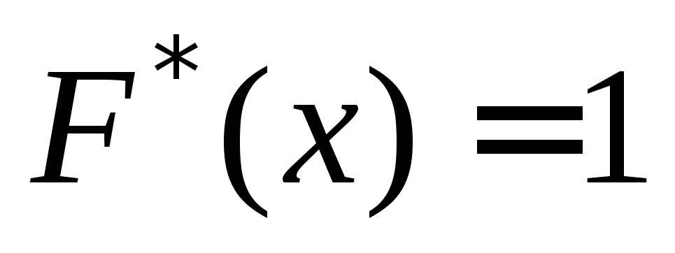
3) If is the smallest option, then = 0 for, if is the largest option, then = 1 for.

The empirical distribution function of the sample is used to estimate the theoretical distribution function of the general population.

Example... Let's construct an empirical function for the distribution of the sample:

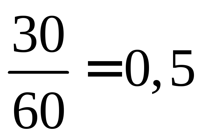
Find the sample size: 12 + 18 + 30 = 60. The smallest option is 2, therefore = 0 for x £ 2. The value of x<6, т.е. , наблюдалось 12 раз, следовательно, =12/60=0,2 при 2< x £6. Аналогично, значения X < 10, т.е. и наблюдались 12+18=30 раз, поэтому =30/60 =0,5 при 6< x £10. Так как x=10 – наибольшая варианта, то =1 при x>10.Thus, the sought empirical function has the form:

The most important properties of statistical estimates

Let it be required to study some quantitative feature of the general population. Let us assume that from theoretical considerations it was possible to establish which one the distribution has a characteristic and it is necessary to evaluate the parameters by which it is determined. For example, if the trait under study is normally distributed in the general population, then you need to estimate the mathematical expectation and standard deviation; if the feature has a Poisson distribution, then it is necessary to estimate the parameter l.

Usually, only sample data are available, for example, values ​​of a quantitative characteristic obtained as a result of n independent observations. Considering as independent random variables, we can say that to find a statistical estimate of an unknown parameter of a theoretical distribution means to find a function of the observed random variables, which gives an approximate value of the estimated parameter. For example, to estimate the mathematical expectation of a normal distribution, the role of a function is played by the arithmetic mean

In order for statistical estimates to give correct approximations of the estimated parameters, they must satisfy certain requirements, among which the most important are the requirements unbiasedness and consistency estimates.

Let be a statistical estimate of the unknown parameter of the theoretical distribution. Let an estimate be found for a sample of size n. Let's repeat the experience, i.e. we extract from the general population another sample of the same size and, according to its data, we obtain a different estimate. Repeating the experiment many times, we get different numbers. The score can be viewed as a random variable, and the numbers as its possible values.

If the estimate gives an approximate value in abundance, i.e. each number is greater than the true value, then, as a consequence, the mathematical expectation (average value) of the random variable is greater than:. Similarly, if gives the estimate with a disadvantage then.

Thus, the use of a statistical estimate, the mathematical expectation of which is not equal to the parameter being estimated, would lead to systematic (one-digit) errors. If, on the contrary, then this guarantees against systematic errors.

Unbiased is called a statistical estimate, the mathematical expectation of which is equal to the estimated parameter for any sample size.

Displaced is an estimate that does not satisfy this condition.

The unbiasedness of the estimate does not yet guarantee a good approximation for the parameter being estimated, since the possible values ​​may be very scattered around its mean, i.e. variance can be significant. In this case, the estimate found from the data of one sample, for example, may turn out to be significantly distant from the mean value, and hence from the estimated parameter itself.

Effective is a statistical estimate that, for a given sample size n, has smallest possible variance .

When considering samples of large size, the requirement is imposed on statistical estimates consistency .

Wealthy is a statistical estimate that, for n® ¥, tends in probability to the parameter being estimated. For example, if the variance of the unbiased estimate tends to zero as n® ¥, then this estimate is also consistent.

Determination of the empirical distribution function

Let $ X $ be a random variable. $ F (x) $ - distribution function of the given random variable. We will carry out $ n $ experiments on a given random variable under the same independent conditions. In this case, we get a sequence of values ​​$ x_1, \ x_2 \ $, ..., $ \ x_n $, which is called a selection.

Definition 1

Each value of $ x_i $ ($ i = 1,2 \ $, ..., $ \ n $) is called a variant.

One of the estimates of the theoretical distribution function is the empirical distribution function.

Definition 3

The empirical distribution function $ F_n (x) $ is a function that determines for each value of $ x $ the relative frequency of the event $ X \

where $ n_x $ is the number of options less than $ x $, $ n $ is the sample size.

The difference between the empirical function and the theoretical one is that the theoretical function determines the probability of the event $ X

Properties of the empirical distribution function

Let us now consider several basic properties of the distribution function.

The range of values ​​of the function $ F_n \ left (x \ right) $ is the segment $$.

$ F_n \ left (x \ right) $ non-decreasing function.

$ F_n \ left (x \ right) $ is a left continuous function.

$ F_n \ left (x \ right) $ is a piecewise constant function and increases only at the points of values ​​of the random variable $ X $

Let $ X_1 $ be the smallest and $ X_n $ the largest option. Then $ F_n \ left (x \ right) = 0 $ for $ (x \ le X) _1 $ and $ F_n \ left (x \ right) = 1 $ for $ x \ ge X_n $.

Let us introduce a theorem that connects the theoretical and empirical functions.

Theorem 1

Let $ F_n \ left (x \ right) $ be the empirical distribution function, and $ F \ left (x \ right) $ the theoretical distribution function of the general sample. Then the equality holds:

\ [(\ mathop (lim) _ (n \ to \ infty) (| F) _n \ left (x \ right) -F \ left (x \ right) | = 0 \) \]

Examples of tasks for finding the empirical distribution function

Example 1

Let the distribution of the sample have the following data recorded using a table:

Picture 1.

Find the sample size, draw up an empirical distribution function and plot it.

Sample size: $ n = 5 + 10 + 15 + 20 = $ 50.

By property 5, we have that for $ x \ le 1 $ F_n \ left (x \ right) = 0 $, and for $ x> 4 $ $ F_n \ left (x \ right) = 1 $.

The value of $ x

The value of $ x

The value of $ x

Thus, we get:

Figure 2.

Figure 3.

Example 2

From the cities of the central part of Russia, 20 cities were randomly selected for which the following data on the cost of travel in public transport were obtained: 14, 15, 12, 12, 13, 15, 15, 13, 15, 12, 15, 14, 15, 13 , 13, 12, 12, 15, 14, 14.

Draw up an empirical distribution function for a given sample and build its graph.

Let's write the sample values ​​in ascending order and calculate the frequency of each value. We get the following table:

Figure 4.

Sample size: $ n = $ 20.

By property 5, we have that for $ x \ le 12 $ F_n \ left (x \ right) = 0 $, and for $ x> 15 $ $ F_n \ left (x \ right) = 1 $.

The value of $ x

The value of $ x

The value of $ x

Thus, we get:

Figure 5.

Let's plot the empirical distribution:

Figure 6.

Originality: $ 92.12 \% $.

Learn what an empirical formula is. In chemistry, EP is the simplest way to describe a compound - in fact, it is a list of elements that form a compound, taking into account their percentage. It should be noted that this simplest formula does not describe order atoms in a compound, it simply indicates what elements it consists of. For example:

• Compound consisting of 40.92% carbon; 4.58% hydrogen and 54.5% oxygen will have the empirical formula C 3 H 4 O 3 (an example of how to find the EF of this compound will be discussed in the second part).

As you know, the distribution law of a random variable can be specified in various ways. A discrete random variable can be specified using a distribution series or an integral function, and a continuous random variable - using either an integral or a differential function. Let's consider selective analogs of these two functions.

Let there be a sample set of values ​​of some random volume and each option from this aggregate is assigned its frequency. Let further, - some real number, and - the number of sampled values ​​of a random variable
less . Then the number is the frequency of the values ​​of the quantity observed in the sample X less , those. the frequency of occurrence of the event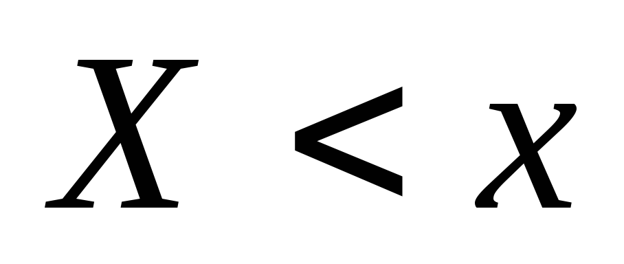
... When it changes x in the general case, the quantity ... This means that the relative frequency is an argument function ... And since this function is found according to sample data obtained as a result of experiments, it is called selective or empirical.

Definition 10.15. Empirical distribution function(the distribution function of the sample) is called the function
determining for each value x relative frequency of the event
.

(10.19)

In contrast to the empirical distribution function of the sample, the distribution function F(x) of the general population is called theoretical distribution function... The difference between them is that the theoretical function F(x) determines the likelihood of an event
, and empirical - the relative frequency of the same event. Bernoulli's theorem implies

,
(10.20)

those. at large probability
and the relative frequency of the event
, i.e.
differ little from one another. This already implies the expediency of using the empirical distribution function of the sample for an approximate representation of the theoretical (integral) distribution function of the general population.

Function
and
have the same properties. This follows from the definition of the function.

Properties
:

Example 10.4. Construct an empirical function for a given sample distribution:

Decision: Find the sample size n= 12 + 18 + 30 = 60. Smallest option
, hence,
at
... Value
, namely
was observed 12 times, therefore:

=
at
.

Value x< 10, namely
and
were observed 12 + 18 = 30 times, therefore,
=
at
... When

.

The required empirical distribution function:

=

Schedule
is shown in Fig. 10.2

R
is. 10.2

Control questions

1. What are the main tasks that mathematical statistics solve? 2. General and sample population? 3. Give a definition of the sample size. 4. What samples are called representative? 5. Errors of representativeness. 6. The main methods of sampling. 7. Concepts of frequency, relative frequency. 8. The concept of a statistical series. 9. Write down the Sturges formula. 10. Formulate the concepts of sample range, median and mode. 11. Frequency polygon, histogram. 12. The concept of a point estimate of the sample population. 13. Biased and unbiased point estimate. 14. Formulate the concept of the sample mean. 15. Formulate the concept of sample variance. 16. Formulate the concept of the sample standard deviation. 17. Formulate the concept of the sample coefficient of variation. 18. Formulate the concept of sample geometric mean.