Characteristics of the binomial distribution. Binomial distribution
Of course, when calculating the cumulative distribution function, it should be used by the mentioned binder and beta-distribution. This method is knowingly better than immediate summation when N\u003e 10.
In classical statistics textbooks, formulas based on limit theorems (such as Moava-Laplace formula) are often recommended to obtain binomial distribution values. It should be noted that with a purely computing point of view The value of these theorems is close to zero, especially now, when almost every table is a powerful computer. The main disadvantage of the above approximations is their completely insufficient accuracy at N values \u200b\u200btypical of most applications. No less disadvantage is the absence of any clear recommendations on the applicability of one or another approximation (only asymptotic wording is given in standard texts, they are not accompanied by accuracy estimates and, therefore, are not very useful). I would say that both formulas are suitable only for n< 200 и для совсем грубых, ориентировочных расчетов, причем делаемых “вручную” с помощью статистических таблиц. А вот связь между биномиальным распределением и бета-распределением позволяет вычислять биномиальное распределение достаточно экономно.
I do not consider here the task of searching for quantile: it is trivial for discrete distributions, and in those tasks where such distributions arise, it is usually not relevant. If quantil will still be needed, I recommend that you reformulate the task to work with p-values \u200b\u200b(observed substances). Here is an example: when implementing some of the current algorithms at each step, it is required to check the statistical hypothesis about the binomial random variable. According to a classic approach at each step, it is necessary to calculate the statistics of the criterion and compare its value with the boundary of the critical set. Since, however, the algorithm is broken, it is necessary to determine the boundary of the critical set every time again (after all, from step to step, the sample volume changes) that there is no integrally increases time costs. A modern approach recommends computing observed significance and compare it with a trustful probability, saving on searching for quantile.
Therefore, in the codes below, there is no reverse function calculation, instead the REV_BINOMIALDF function is shown, which calculates the probability P of success in a separate test on a given amount of N testing, the number of M success in them and the probability of these M success. It uses the above-mentioned bond between the binomial and beta distribution.
In fact, this feature allows you to get boundaries of trust intervals. In fact, we assume that in N binomial tests we received M success. As is known, the left limit of the bilateral confidence interval for the parameter p with the confidence level is 0, if M \u003d 0, and for the solution of the equation  . Similarly, the right boundary is 1, if M \u003d n, and for the solution of the equation
  . From here it follows that to search for the left border, we must solve relative to the equation
  , and to find the right - equation
  . They are solved in the BINOM_LEFTCI and BINOM_RIGHTCI functions that return the upper and lower boundaries of the two-way confidence interval, respectively.
I want to note that if you do not need absolutely incredible accuracy, then with quite large N, it is possible to take advantage of the following approximation [B.L. Van der Warden, mathematical statistics. M: IL, 1960, ch. 2, sec. 7]:  where G is a quantile normal distribution. The value of this approximation is that there are very simple approximations, allowing you to calculate the quantilation of the normal distribution (see the text on the calculation of the normal distribution and the corresponding section of this reference book). In my practice (mainly, with n\u003e 100), this approximation gave about 3-4 characters, which is usually quite enough.
For computation using the following codes, Betadf.h files will be required, betadf.cpp (see the section on beta distribution), as well as loggamma.h, loggamma.cpp (see Appendix A). You can also see an example of using functions.
File binomialdf.h.
| #ifndef __binomial_h__ #include "Betadf.h" Double Binomialdf (Double Trials, Double Successes, Double P); / * * Let there be "trials" of independent observations * with the probability of "p" of success in each. * The probability of B (successes | trials, p) is calculated that the number * success is concluded between 0 and "Successes" (inclusive). * / Double Rev_BinomiaLDF (Double Trials, Double Successes, Double Y); / * * Suppose Let the probability of a y occuring at least M success * in trials tests of the Bernoulli scheme. The function finds the probability P * success in a separate test. * * In the calculations, the following ratio is used * * 1 - P \u003d Rev_Beta (Trials-Successes | Successes + 1, Y). * / Double Binom_leftci (Double Trials, Double Successes, Double Level); / * Let there be "trials" of independent observations * with the probability of "p" success in each * and the number of success is "successes". * The left limit of the bilateral confidence interval * is calculated with the level of significance Level. * / Double Binom_rightci (Double N, Double Successes, Double Level); / * Let there be "trials" of independent observations * with the probability of "p" success in each * and the number of success is "successes". * The right boundary of the bilateral confidence interval * is calculated with the level of importance level. * / #endif / * EndS #ifndef __binomial_h__ * / |
File binomialdf.cpp.
| / ************************************************* ********** / / * Binomial distribution * / / ******************************** *************************** / #Include. |
The theory of probability is invisibly present in our lives. We do not pay attention to it, but each event in our lives has one probability. Taking into account the huge number of options for the development of events, it becomes necessary to determine the most likely and least likely of them. It is convenient to analyze such probabilistic data graphically. In this we can help the distribution. Binomial is one of the easiest and most accurate.
Before proceeding directly to mathematics and theory of probability, let's deal with those who first came up with such a type of distribution and what is the history of the development of the mathematical apparatus for this concept.
History
The concept of probability is known since ancient times. However, the ancient mathematicians did not attach particular importance to it and were able to lay only the basics for the theory, which subsequently became theory of probability. They created some combinatorial methods that strongly helped those who later created and developed the theory itself.
In the second half of the seventeenth century, the formation of basic concepts and methods of probability theory began. Random variables were introduced, methods for calculating the likelihood of simple and some complex independent and dependent events. Dictated such interest in random values \u200b\u200band probabilities was gambling: every person wanted to know what chances he had to win in the game.
The next step was the application in the theory of the probability of mathematical analysis methods. This was engaged in prominent mathematicians, such as Laplace, Gauss, Poisson and Bernoulli. It was they who advanced this region of mathematics to a new level. It was James Bernoulli that opened the binomial law of distribution. By the way, as we later find out, on the basis of this discovery, several more, which allowed to create the law of normal distribution and many more others.
Now, before you begin to describe the distribution of binomial, we are a little refreshing in the memory of the concept of probability theory, probably already forgotten from school bench.
Fundamentals of probability theory
We will consider such systems as a result of which only two exodus are possible: "success" and "not success". It is easy to understand on the example: we throw the coin, fading what the rush will fall out. The probability of each of the possible events (the rush will fall - "success", the eagle will fall out - "not success") are equal to 50 percent with the ideal balance of the coin and the absence of other factors that may affect the experiment.
It was the easiest event. But there are also complex systems in which successive actions are performed, and the probabilities of the outcomes of these actions will be different. For example, consider such a system: in a box, the contents of which we cannot see, lie six completely identical balls, three pairs of blue, red and white colors. We must get at random few balls. Accordingly, pulling out one of the white balls, we reducing the probability that the white ball will also come to us. This happens because the number of objects in the system changes.
In the next section, we consider more complex mathematical concepts, closely applied to what they mean the words "normal distribution", "binomial distribution" and the like.

Elements of mathematical statistics
In statistics, which is one of the applications of probability theory, there are many examples when data for analysis is not explicitly. That is, not in the numerical, but in the form of division on features, for example, by sex. In order to apply a mathematical apparatus to such data and make some conclusions from the results obtained, the source data in the numeric format is required. As a rule, for the implementation of this, a positive outcome is assigned a value of 1, and negative - 0. Thus, we obtain statistical data that can be analyzed using mathematical methods.
The next step in understanding what the binomial distribution of a random variable is determining the dispersion of random variable and mathematical expectation. Talk to this in the next section.

Expected value
In fact, it is easy to understand what mathematical expectation is easy. Consider the system in which there are many different events with your different probabilities. The mathematical expectation will be called the value equal to the amount of the values \u200b\u200bof these events (and the mathematical form we spoke in the past section) on the likelihood of their implementation.
The mathematical expectation of the binomial distribution is calculated by the same scheme: we take the value of a random variable, multiply it on the likelihood of a positive outcome, and then we summarize the data obtained for all values. It is very convenient to present these data graphically - it is better that the difference between the mathematical expectations of different quantities is perceived.
In the next section, we will tell you a little about another concept - dispersion of a random variable. It is also closely associated with such a concept as a binomial probability distribution, and is its characteristic.

Dispersion of binomial distribution
This value is closely related to the previous one and also characterizes the distribution of statistical data. It is an average square of deviations of values \u200b\u200bfrom their mathematical expectation. That is, the dispersion of a random variable is the sum of the squares of the differences between the value of the random variable and its mathematical expectation, multiplied by the likelihood of this event.
In general, that's all we need to know about the dispersion to understand what the binomial distribution of probabilities is. Now let's get directly to our main topic. Namely, what lies for this in the appearance of a rather complex phrase "Binomial distribution law".

Binomial distribution
Let's figure out for a start why this is a binomial distribution. It comes from the word "bin". Maybe you heard about Newton's Binoma - such a formula with which you can decompose the sum of two any numbers a and b to any non-negative degree n.
As you probably have already guessed, the formula of the Binoma Newton and the formula of the binomial distribution is almost the same formulas. It is only an exception that the second is applied for specific quantities, and the first is only a common mathematical tool whose applications can be different in practice.
Distribution formulas
The binomial distribution function can be recorded as the sum of the following members:
(n! / (n - k)! k!) * p k * q n-k
Here n is the number of independent random experiments, the number of successful outcomes, q - the number of unsuccessful outcomes, k is the experiment number (may take values \u200b\u200bfrom 0 to n) ,! - the designation of the factorial, such a function, the value of which is equal to the product of all numbers going to it (for example, for the number 4: 4! \u003d 1 * 2 * 3 * 4 \u003d 24).
In addition, the binomial distribution function can be recorded as an incomplete beta function. However, this is a more complex definition, which is used only when solving complex statistical problems.
The binomial distribution, the examples of which we considered above are one of the simplest types of distributions in the theory of probability. There is also a normal distribution, which is one of the types of binomial. It is used most often, and most simply in the calculations. There is also the distribution of Bernoulli, the distribution of Poisson, the conditional distribution. All of them characterize graphically areas of the likelihood of one or another process under different conditions.
In the next section, consider aspects regarding the use of this mathematical apparatus in real life. At first glance, of course, it seems that this is another mathematical thing, which, as usual, does not find applications in real life, and at all is not needed by anyone, except for the mathematicians themselves. However, this is not the case. After all, all types of distributions and their graphic representations were created exclusively under practical purposes, and not as whims of scientists.

Application
Of course, the most important application of the distribution is found in statistics, because there is a comprehensive analysis of the set of data. As practice shows, very many data arrays have about the same distributions of quantities: critical areas of very low and very high values, as a rule, contain fewer items than the average values.
Analysis of large data arrays is required not only in statistics. It is indispensable, for example, in physical chemistry. In this science, it is used to determine many values \u200b\u200bthat are associated with random oscillations and movements of atoms and molecules.
In the next section, we will deal with how important the use of such statistical concepts as binomial the distribution of a random variable in everyday life for us with you.

Why do I need it?
Many ask themselves such a question when it comes to mathematics. And by the way, mathematics is not in vain called the Queen of Science. It is the basis of physics, chemistry, biology, economics, and in each of these sciences is used including any distribution: whether it is a discrete binomial distribution, or normal, no matter. And if we get better to the world around the world, we will see that mathematics is applied everywhere: in everyday life, at work, and even human relations can be submitted in the form of statistical data and analyze their analysis (so, by the way, they make those who work in special organizations involved in collecting information).
Now let's talk a little about what to do if you need to know on this topic much more than what we have outlined in this article.
That information that we gave in this article are far from complete. There are many nuances regarding what form can take distribution. The binomial distribution, as we have already found out, is one of the main species on which all mathematical statistics and probability theory are based.
If it became interesting to you, or in connection with your work, you need to know on this topic much more, you will need to explore specialized literature. Start follows from the university course of mathematical analysis and travel there to the section of the theory of probability. Knowledge of the rows will also be useful, because the binomial distribution of probabilities is nothing more than a series of consecutive members.
Conclusion
Before completing the article, we would like to tell another interesting thing. It concerns the topics of our article and the whole mathematics as a whole.
Many people say that mathematics is useless science, and nothing from what they took place at school, they were not useful. But knowledge is never superfluous, and if something is not useful to you in life, it means that you just don't remember this. If you have knowledge, they can help you, but if they are not, then you can't wait for help from them.
So, we considered the concept of binomial distribution and all the associated definitions and talked about how it applies to our life with you.
Consider the implementation of the Bernoulli scheme, i.e. A series of repeated independent tests is available, in each of which this event A has the same probability that does not depend on the test number. And for each test there are only two outages:
1) Event A - Success;
2) Event - fail
with constant probabilities
We introduce a discrete random amount x - "The number of events and p Tests "and find the law of distribution of this random variable. X can make values
Probability ![]() that the random variable will take a value x K. Located by Bernoulli Formula
that the random variable will take a value x K. Located by Bernoulli Formula
The law of distribution of the discrete random variable determined by the Bernoulli formula (1) is called binomial distribution law. Permanent p and r (q \u003d 1-P)included in formula (1) are called binomial distribution parameters.
The name "binomial distribution" is associated with the fact that the right side in equality (1) is a general member of the decomposition of Newton's Binoma, i.e.
(2)
And since p + Q \u003d 1, the right side of equality (2) is equal to 1
It means that
 (4)
(4)
In equality (3), the first member q N. The right part means the likelihood that in p Tests event and never will appear, second member ![]() the likelihood that event A will appear once, the third dick is the likelihood that the event A will appear twice and finally, the last member p P. - the likelihood that event A will appear exactly p time.
the likelihood that event A will appear once, the third dick is the likelihood that the event A will appear twice and finally, the last member p P. - the likelihood that event A will appear exactly p time.
The binomial distribution law of the discrete random variable is represented as a table:
| H. | 0 | 1 | … | k. | … | n. |
| R | q N. | … | … | p P. |
The main numeric characteristics of the binomial distribution:
1) mathematical expectation ![]() (5)
(5)
2) Dispersion ![]() (6)
(6)
3) secondary quadratic deviation ![]() (7)
(7)
4) the most suitable number of events k 0 - This is the number with the specified p corresponds to the maximum binomial probability
For specified p and r This number is determined by inequalities
![]() (8)
(8)
if the number pR + R. is not integer then k 0 Equally a whole part of this number, if pR + R. - integer, then k 0 He has two meanings
The binomial law of probability distribution is applied in the theory of shooting, in theory and practice of statistical control of product quality, in the theory of mass service, in reliability theory, etc. This law can be applied in all cases when there is a sequence of independent tests.
Example 1:Quality testing is established that out of each 100 devices do not have defects 90 pieces on average. Make a binomial law of probability distribution of the number of high-quality devices from acquired at random 4.
Decision:Event A - the appearance of which is checked by this - "Acquired at random device quality". Under the condition of the problem, the main parameters of the binomial distribution:
The random value X is the number of high-quality devices made of 4, which means the values \u200b\u200bof x-try the likelihood of x values \u200b\u200bby formula (1):

Thus, the value of the distribution of the amount of X is the number of high-quality instruments made of 4:
| H. | 0 | 1 | 2 | 3 | 4 |
| R | 0,0001 | 0,0036 | 0,0486 | 0,2916 | 0,6561 |
To check the correctness of the distribution construct, check why the sum of probabilities is equal
Answer:Distribution law
| H. | 0 | 1 | 2 | 3 | 4 |
| R | 0,0001 | 0,0036 | 0,0486 | 0,2916 | 0,6561 |
Example 2:The treatment method used leads to recovery in 95% of cases. Five patients applied this method. Find the most numerical characteristics of the random variable x - the number of recovered from 5 patients used this method.
Consider the binomial distribution, we calculate its mathematical expectation, dispersion, fashion. Using the MS Excel function Binomesp (), we construct graphs of the distribution function and probability density. We will evaluate the parameter of the distribution P, the mathematical expectation of the distribution and standard deviation. We will also consider the distribution of Bernoulli.
Definition . Let them be held N. Tests, in each of which only 2 events may occur: the event "success" with probability P. or the event "failure" with probability Q. \u003d 1-P (so-called Bernoulli Scheme, Bernoulli. trials.).
The probability of obtaining exactly X. Successes in these N. Tests are equal to:
The number of success in the sample X. is a random value that has Binomial distribution (eng. Binomial Distribution.) P. and N. – are the parameters of this distribution.
Recall that for use Bernoulli schemes and correspondingly Binomial distribution The following conditions must be completed:
- each test must have exactly two outcome, conditionally referred to as "success" and "failure."
- the result of each test should not depend on the results of previous tests (test independence).
- probability of success P. Must be constant for all tests.
Binomial distribution in MS Excel
In MS Excel, starting in 2010, for there is a BINOM function (), the English name - binom.dist (), which allows you to calculate the likelihood that in the sample will be smooth H. "Successes" (i.e. The function of the probability density p (x), see the formula above), and integral distribution function (the likelihood that in the sample will be X. or less "success", including 0).
Before MS Excel 2010, Excel had a binomap () function, which also allows us to calculate Distribution function and probability density P (x). Binomap () is left in MS Excel 2010 for compatibility.
The example file shows graphs Distribution of probability and .
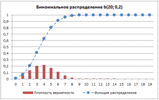
Binomial distribution Has notation B. ( N. ; P.) .
Note : For building integral distribution function Ideal fit diagram Schedule for Distribution distribution – Histogram with grouping . Read more about Building Charts Read the article Main types of diagrams.
Note : For ease of writing, the formulas in the example file created names for parameters Binomial distribution : n and p.

The example file provides various probability calculations using MS Excel functions:
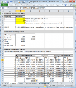
As can be seen in the picture above, it is assumed that:
- In an infinite set, from which the sample is made, contains 10% (or 0.1) of the suitable elements (parameter P. , the third argument of the function \u003d bin.Rasp ())
- To calculate the likelihood that in the sample of 10 elements (parameter N. The second function argument) will be exactly 5 suitable elements (first argument), you need to record the formula: \u003d Binomasp (5; 10; 0,1; lies)
- The last, fourth element, set \u003d false, i.e. Returns the value of the function Distribution distribution .
If the value of the fourth argument \u003d truth, then the bin function () returns the value integral distribution function or simply Distribution function . In this case, it is possible to calculate the likelihood that in the sample the number of suitable elements will be from a specific range, for example, 2 or less (including 0).
To do this, you need to write down the formula: \u003d Binom.RP (2; 10; 0.1; truth)
Note : With the nenet value x ,. For example, the following formulas will return the same value: \u003d Bin. 2 ; 10; 0.1; TRUE) \u003d Bin. 2,9 ; 10; 0.1; TRUE)
Note : In the example file probability density and Distribution function Also calculated using the definition and function of NUMCOMB ().
Distribution indicators
IN Example File on Sheet Example There are formulas for calculating some distribution indicators:
- \u003d n * p;
- (standard deviation square) \u003d n * p * (1-p);
- \u003d (n + 1) * p;
- \u003d (1-2 * p) * root (n * p * (1-p)).
Withdraw the formula mathematical expectation Binomial distribution Using Bernoulli scheme .
By definition, the random value x in Bernoulli scheme (Bernoulli Random Variable) has Distribution function :

This distribution is called Distribution of Bernoulli .
Note : Distribution of Bernoulli - Private case Binomial distribution with parameter n \u003d 1.
Let us generate 3 array of 100 numbers with different probabilities of success: 0.1; 0.5 and 0.9. To do this in the window Generation of random numbers Set the following parameters for each probability P:

Note : If you set the option Random dispersion ( Random SEED) You can choose a specific random set of generated numbers. For example, by setting this option \u003d 25, it can be generated on different computers the same sets of random numbers (unless, of course, other distribution parameters are coincided). The option value can take entire values \u200b\u200bfrom 1 to 32 767. Options name Random dispersion can confuse. It would be better to translate it as Set number with random numbers .
As a result, we will have 3 columns of 100 numbers, on the basis of which you can, for example, evaluate the likelihood of success. P. according to the formula: Number of success / 100 (cm. File Example Leaf GenerationBurly).
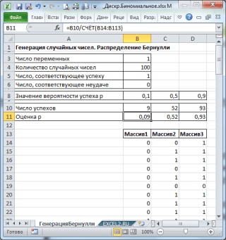
Note : For Distribution of Bernoulli With P \u003d 0.5, you can use the formula \u003d rationing (0; 1), which corresponds.
Generation of random numbers. Binomial distribution
Suppose that 7 defective products have been discovered in the sample. This means that the situation is "very likely" that the share of defective products has changed P. which is the characteristic of our production process. Although this situation is "very likely", but there is a chance (alpha risk, the error of the 1st kind, "false alarm"), which is still P. It remained unchanged, and the increased number of defective products is due to the random of sampling.
As can be seen in the figure below, 7 is the number of defective products, which is permissible for the process with P \u003d 0.21 with the same value Alpha . This serves as an illustration that when the threshold value of defective products is exceeded in the sample, P. "Most likely" increased. The phrase "most likely" means that there is only a 10% probability (100% -90%) that the deviation of the share of defective products above the threshold is caused by only the causes.

Thus, the exceeding the threshold number of defective products in the sample can be a signal that the process is upset and began to produce b about Spent percentage of defective products.
Note : Before MS Excel 2010 in Excel there was a CRTBIN () function (), which is equivalent to binomes (). Cretebin () is left in MS Excel 2010 and above for compatibility.
Communication of binomial distribution with other distributions
If the parameter N. Binomial distribution tends to infinity, and P. tends to 0, then in this case Binomial distribution It can be approximated. Conditions can be formulated when the approximation Poisson distribution works good:
- P. (the less P. and more N. , the nearest approximation);
- P. >0,9 (considering that Q. =1- P. , calculations in this case should be done through Q. (but H. Need to replace on N. - X.). Therefore Q. and more N. , the approximation is more accurate).
At 0.110. Binomial distribution You can approximate.
In turn, Binomial distribution can serve as a good approximation when the size of the totality n Hypergeometric distribution Much more sample sampling N (i.e., N \u003e\u003e N or N / N. More about the connection of the above distributions, you can read in the article. There are also examples of approximation, and conditions are explained when it is possible with what accuracy.
Council : On other MS Excel distributions can be found in the article.
Chapter 7.
Specific laws of distribution of random variables
Types of laws of distribution of discrete random variables
Let the discrete random value can take values h. 1 , h. 2 , …, x N..... The probabilities of these values \u200b\u200bcan be calculated according to various formulas, for example, using the basic theorems of probability theory, Bernoulli formulas or by some other formulas. For some of these formulas, the distribution law has its name.
The most common laws of distribution of discrete random variance are binomial, geometric, hypergeometric, Poisson distribution law.
Binomial distribution law
Let it be produced n. independent tests, in each of which an event may appear or do not appear BUT. The likelihood of this event in each single test is constant, does not depend on the test number and equal r=R(BUT). Hence the probability of no event BUT In each test is also constant and equal q.=1–r. Consider a random amount H. equal to the number of events BUT in n. Tests. Obviously, the values \u200b\u200bof this value are equal
h. 1 \u003d 0 - Event BUT in n. Tests did not appear;
h. 2 \u003d 1 - Event BUT in n. Tests appeared once;
h. 3 \u003d 2 - Event BUT in n. Tests appeared twice;
…………………………………………………………..
x N. +1 = n. - Event BUT in n. Tests appeared n. time.
The probabilities of these values \u200b\u200bcan be calculated by the Bernoulli formula (4.1):
where to=0, 1, 2, …, N. .
Binomial distribution law H.equal to the number of success in n. Bernoulli tests, with probability of success r.
So, the discrete random value has a binomial distribution (or distributed according to the binomial law) if its possible values \u200b\u200bare 0, 1, 2, ... n., and corresponding probabilities are calculated by formula (7.1).
Binomial distribution depends on two parameters r and n..
A number of distribution of a random variable, distributed according to the binomial law, has the form:
| H. | … | k. | … | n. | ||
| R | | … | … | |
Example 7.1 . There are three independent target shots. The probability of entering each shot is 0.4. Random value H. - the number of hits in the target. Build her number of distribution.
Decision. Possible values \u200b\u200bof random variable H. are h. 1 =0; h. 2 =1; h. 3 =2; h. 4 \u003d 3. We find the corresponding probabilities using the Bernoulli formula. It is easy to show that the use of this formula here is quite justified. Note that the probability of not entering the target at one shot will be 1-0.4 \u003d 0.6. Receive

A number of distribution is as follows:
| H. | ||||
| R | 0,216 | 0,432 | 0,288 | 0,064 |
It is easy to verify that the sum of all probabilities is equal to 1. Random number itself H. Distributed by binomial law. ■.
We find the mathematical expectation and dispersion of a random variable distributed according to the binomial law.
When solving Example 6.5 it was shown that the mathematical expectation of the number of events appearances BUT in n. independent tests if the probability of appearance BUT In each test is constant and equal rwell n.· r
In this example, a random variable, distributed according to the Binomial Law. Therefore, the solution of Example 6.5 is essentially the proof of the following theorem.
Theorem 7.1. The mathematical expectation of the discrete random variable distributed according to the binomial law is equal to the product of the number of tests on the likelihood of "success", i.e. M.(H.)= N.· r.
Theorem 7.2.The dispersion of the discrete random variable, distributed according to the binomial law, is equal to the product of the number of tests on the likelihood of "success" and on the likelihood of "failure", i.e. D.(H.)= NPQ.
Asymmetry and excess of a random variable, distributed according to the binomial law, are determined by formulas
These formulas can be obtained by using the concept of initial and central moments.
The binomial distribution law underlies many real situations. For large values n. Binomial distribution can be approximated by other distributions, in particular by the help of Poisson distribution.
Poisson distribution
Let it be N.bernoulli tests, with the number of tests n. Great enough. Previously shown that in this case (if more likely r events BUT very small) to find the likelihood that the event BUT to appear t. Once in the tests you can use the Formula of Poisson (4.9). If a random value H. means the number of events BUT in n.bernoulli tests, the probability that H. Take a value k. can be calculated by the formula
 , (7.2)
where λ = nR.
Law of the distribution of Poissoncalled the distribution of discrete random variable H.for which the possible values \u200b\u200bare whole non-negative numbers, and probabilities r T. These values \u200b\u200bare found by formula (7.2).
Value λ = nRcalled parameterpoisson distribution.
A random variable distributed by the law of Poisson can take an infinite set of values. As for this distribution probability r The appearance of the event in each test is small, this distribution is sometimes called the law of rare phenomena.
A number of distribution of a random variable distributed by the law of Poisson has the form
| H. | … | t. | … | ||||
| R | … | … |
It is not difficult to make sure that the probability amount of the second string is 1. To do this, it is necessary to remember that the function can be decomposed into a row of Macrolore, which converges for any h.. In this case we have
 . (7.3)
As noted, the Law of Poisson in certain limiting cases replaces the binomial law. As an example, you can bring a random amount H., the values \u200b\u200bof which are equal to the number of failures for a certain period of time with repeated use of the technical device. It is assumed that this is a high reliability device, i.e. The probability of failure at one application is very small.
In addition to such margins, in practice there are random variables distributed under the Poisson law that are not related to the binomial distribution. For example, Poisson's distribution is often used when they deal with the number of events that appear in the time of time (the number of calls to the telephone exchange within an hour, the number of cars arrived on the car washing during the day, the number of stops of machines per week, etc. .). All these events should form, the so-called flow of events, which is one of the basic concepts of mass maintenance theory. Parameter λ characterizes the average intensity of the flow of events.
Example 7.2 . The faculty has 500 students. What is the likelihood that September 1 is the birthday for three students of this faculty?
Decision . Since the number of students n.\u003d 500 is large enough and r - The probability of the first of September is born to any of the students equal, i.e. enough small, then we can assume that a random value H. - The number of students born first of September is distributed under Poisson's law with a parameter λ = nP.\u003d \u003d 1.36986. Then, by formula (7.2) we get
Theorem 7.3.Let a random value H. Distributed by the law of Poisson. Then its mathematical expectation and dispersion are equal to each other and equal to the value of the parameter λ . M.(X.) = D.(X.) = λ = nP..
Evidence. By determining the mathematical expectation, using formula (7.3) and a number of distribution of a random variable distributed by the law of Poisson, we obtain
Before finding the dispersion, we will find the mathematical expectation of the square of the random variable under consideration. Receive

From here, by definition of the dispersion, we get
Theorem is proved.
Applying the concepts of the initial and central moments, it can be shown that for a random variable, distributed under the law of Poisson, the coefficients of asymmetry and the excesses are determined by formulas
It is not difficult to understand that, since in the semantic content of the parameter λ = nP. It is positive, then asymmetry and excheses are always positive asymmetry and excheses in a random variable.
